
Advanced Simulation Analysis
 |
David van der Spoel 2007 |
|---|---|
| Dept. of Cell and Molecular Biology | |
| Uppsala University | |
| spoel at xray.bmc.uu.se |
|
David van der Spoel 2007 |
|---|---|
| Dept. of Cell and Molecular Biology | |
| Uppsala University | |
| spoel at xray.bmc.uu.se |
In this exercise we will show how to perform some advanced analyses on MD trajectories using standard GROMACS tools and some simple scripts. The obvious aim is to try to reach quantitative agreement with experiment for measured properties, in order to proceed to predict things that have not been, or can not be measured. The topics covered here are NMR relaxation and Hydrogen bond kinetics and thermodynamics. Obviously there are many more analysis tools than what can be tested in a few hours, but there must be something left to discover for yourself.
Background reading for this bit is given below.
| Files | DOI |
|---|---|
| spoel_thesis_chap2.pdf | (contains summary of how to compare experiment to simulation, including introduction into NMR relaxation) |
| tjandra1995a.pdf, tjandra1995a-sup.pdf | Rotational diffusion anisotropy of human ubiquitin from 15N NMR relaxation |
| villa2006a.pdf, villa2006a-sup.pdf | What NMR Relaxation Can Tell Us about the Internal Motion of an RNA Hairpin: A Molecular Dynamics Simulation Study |
| lindorff-larsen2005a.pdf | Simultaneous determination of protein structure and dynamics |
For this exercise we have borrowed a trajectory of a Ubiquitin simulation from Marvin Seibert. Please make a new subdirectory and download the following files (you will need 2Gb free space):
It is always a good idea to check what we really have, so make a pdb file from the tpr (using editconf) and have a look at it using Pymol or VMD.
Now we will try to compute the dynamics of the NH vectors in the molecules with respect to the overall motion, that is, the overall motion has been removed from the trajectory already, and we will investigate only the internal dynamics.
First we will have to define which residues are suited for the analysis. The first residue is charged and hence has three different H atoms connected to the N. The Proline residues (19, 37, 38) don't have a H, so residues 1, 19, 38 and 39 have to be excluded from the analysis. We use the make_ndx to make an appropriate index file. Since this is slightly (only slightly) tedious, we provide the complete command sequence here, for your cutting and pasting pleasure:
make_ndx -f topol.tpr -o nh << EOF
a N | a H
r 1 | r 19 | r 38 | r 39
10 & !11
name 12 NH
del 0-11
q
EOF
The file does now hold a list of atom numbers all the time in the order NH, NH etc. You may want to verify the result using the gmxcheck tool with the -n flag. Now we are ready to rock. We'll use the g_rotacf program with the following flags: -d -n nh -P 2 -f traj. This will give us the autocorrelation of the 2nd order Legendre polynomial of the NH bond vector. This analysis will take a few minutes. View the result with the xmgrace program.
Time for critical reflection. What do you see? Has the curve equilibrated? (Note that the trajectory is 25 ns, but only 12.5 ns is shown). What could be the cause of this? Using xmgrace you can do fit to the curve (Data/Transformations/Non-Linear Curve Fittings). First, create a model with two parameters, and use the following formula: y = a0+(1-a0)*exp(-x/a1), and choose suitable starting parameters (a0 = 0.8, a1 = 100). Press Apply a few times. Does the fit look good? Why not?
Now let's try a four parameter model: y = a0+(1-a0-a2)*exp(-x/a1)+a2*exp(-x/a3), press Apply a couple of times again. Does this look better? What are the relaxation times in this model? How would you interpret this model?
Time to make matters complicated. By redoing the analysis with the -noaver flag you obtain an output file that has all the correlation functions for all NH vectors separately. (Do the analysis now!). Check the results again using xmgrace. Note that each curve now represents one NH vector, numbered in order of the residues. You can redo the curve fitting to one or a few curves to check convergence.
Let's pretend that the simulation gives us perfectly converged results for the dynamics of all NH all vectors. Now we can determine the order parameter S2 by taking the average over the second half of each relaxation curve. Since this is simple, it could be left as an exercise to the reader, but we provide a little perl script that you can download from the link above. If you have done this, run:
./process_rotacf.pl rotacf.xvgThis gives you a new file S2.xvg holding the simulated order parameters for each residue which then should be compared with experiment. The latter can be done using the provided S2exp.xvg where we have copied the experimental values from the paper by Tjandra et al.. Just run xmgrace on both files at the same time. Does it look good? More critical reflection needed here. Now the exercise turns into science, and there are no more easy answers. Good luck!
Background reading for this bit is given below.
For this exercise we will use a number of trajectories due to Erik Wensink et al. containing a 40% Ethanol solution at three different temperatures. You can download a tar file here. Unpack it using tar xvf eth40.tar then you will have a new directory eth40 with three subdirectories corresponding to the temperatures 15, 25 and 35oC.
Now run the following command in all three directories, and make sure you write down the results for the Forward DG:
g_hbond -f traj -s topol -acand choose System in both cases. The program compute the hydrogen bond (HB) autocorrelation function, you can view the ACF (hbac.xvg) using xmgrace. The DG that you are noting down here corresponds to the Gibbs energy of activation for breaking a hydrogen bond. Now create a file where you write two columns, 1/temperature in 1/K and DG/T. Plot this file using xmgrace and compute the regression coefficient (Data/Transformations/Regression), this yields the Enthalpy of activation by the Van 't Hoff equation:
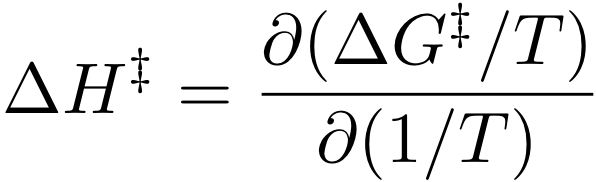
The DHact can be measured by Raman spectroscopy (see paper spoel2006b.pdf for references), however, it is usually measured only for pure liquids. If simulations could reproduce these, and other mixing properties such as energy and density (wensink2003a.pdf) then we could use simulation to fill in the gaps. Unfortunately standard force field like OPLS or GROMOS are not good enough for this yet.
To increase our understanding of the reactive flux correlation we will repeat the steps in Eqn. 3-6 in spoel2006b.pdf. Load one of the files provided in xmgrace: xmgrace -nxy hbac-all.xvg.gz. We will be using the black [c(t)], the green [-K(t)] and the blue [n(t)] curves. Therefore click on the red curve and in the Set Appearance, right click on the second set (s1) and select hide (or kill). Using xmgrace's built-in data analysis we will now derive the rate constants k and k'. Go to (Data/Transformations/Non Linear Curve Fitting) and select the third set (s2), and type the following equation: y = a0*s0.y - a1*s3.y and press Apply a number of times. If you zoom in somewhat you can see that the fit is quite good. According to Luzar2000a.pdf the very first bit in the graph is not well described by the equations, so we take away the first ps from the analysis. Go to (Data/Data Set Operations), select all sets, then select from the Drop Down menu the option Drop Points. Type in the fields 0 and 5 respectively (there are 5 points per ps), and then go back to the Non Linear Curve Fitting dialog box and press apply again. As you'll note the fit gets a lot better this way. Now note down the a0 and a1 constants and explain what they mean. Finally, using Eqn. 6 we can derive the Gibbs activation energy for breaking of the HB.