Theoretical Background

We briefly state the basic working equations in the following, as far as required to understand the program output. For a more detailed treatment of the theory see refs. [76,16,75,77,78] and refs. therein.

The first-order frequency dependent response of the density matrix can be expanded as

$$\sum_{{ai}}^{} \varphi_{{i}}^{} \varphi_{{a}}^{*} \varphi_{{a}}^{} \varphi_{{i}}^{*}$$ (7.1)

The (real) expansion coefficients X_ai and Y_ai are conveniently gathered in a ``super-vector''

$$\left(\vphantom{ \begin{array}{r} X \\ Y \end{array} }\right. \begin{array}{r} X \\ Y \end{array} \left.\vphantom{ \begin{array}{r} X \\ Y \end{array} }\right)$$ (7.2)

on L, the linear space of products of occupied and virtual ground state MOs
$\varphi_{{i}}^{}$(x)$\varphi_{{a}}^{*}$(x') plus their complex conjugates. X and Y describe the first-order change of the ground state MOs due to an external perturbation which is represented by $\ensuremath{\vert P,Q\rangle}$ on L. For example, if an oscillating electric dipole perturbation along the z axis is applied, $\ensuremath{\vert P,Q\rangle} = \ensuremath{\vert\mu_z\rangle}$, where $\ensuremath{\mathbf{\mu}}$ is the electric dipole operator.

Next we define the 2×2 ``super-matrices''

$$\left(\vphantom{ \begin{array}{rr} A & B \\ B & A \end{array} }\right. \begin{array}{rr} A & B \\ B & A \end{array} \left.\vphantom{ \begin{array}{rr} A & B \\ B & A \end{array} }\right) \left(\vphantom{\begin{array}{rr} 1 & 0 \\ 0 & -1 \end{array} }\right. \begin{array}{rr} 1 & 0 \\ 0 & -1 \end{array} \left.\vphantom{\begin{array}{rr} 1 & 0 \\ 0 & -1 \end{array} }\right)$$ (7.3)

where the four-index quantities A and B are the so-called ``orbital rotation Hessians''. Explicit expressions for A and B can be found, e.g., in ref. [16]. The vector $\ensuremath{\vert X,Y\rangle}$ is determined as the solution of the TDHF/TDDFT response problem,

(Λ - ωΔ)| X, Y〉 = - | P, Q〉. (7.4)

If $\ensuremath{\vert X_{\alpha},Y_{\alpha}\rangle}$ arises from an electric dipole perturbation $\ensuremath{\vert\mu_{\alpha}\rangle}$, the electronic dipole polarizability at frequency ω is

α_αβ(ω) = - 〈X_α, Y_α| μ_β〉, (7.5)

α, β∈{x, y, z}. Similarly, if $\ensuremath{\vert m_{\alpha}\rangle}$ is a component of the magnetic dipole moment operator, the optical rotation is [79]

$${\tfrac{{c}}{{3\omega}}}$$ (7.6)

where c is the light velocity.

Excitation energies Ω_n are the poles of the frequency-dependent density matrix response. They are thus the zeros of the operator on the left-hand side of Eq. (7.4),

(Λ - Ω_nΔ)| X_n, Y_n〉 = 0. (7.7)

The corresponding eigenvectors $\ensuremath{\vert X_n,Y_n\rangle}$ are the transition density matrices for a given excitation (also called ``excitation vectors'' in the following). They are required to be normalized according to

〈X_n, Y_n| Δ| X_n, Y_n〉 = 1. (7.8)

Transition moments are evaluated by taking the trace with one-particle operators, e.g.,

$$\boldsymbol\mu \boldsymbol\mu$$ (7.9)

for the electric and

m⁰ⁿ = 〈X_n, Y_n|m〉 (7.10)

for the magnetic transition dipole moments.

The full TDHF/TDDFT formalism is gauge-invariant, i.e., the dipole-length and dipole-velocity gauges lead to the same transition dipole moments in the basis set limit. This can be used as a check for basis set quality in excited state calculations. The TDA can formally be derived as an approximation to full TDHF/TDDFT by constraining the Y vectors to zero. For TDHF, the TDA is equivalent to configuration interaction including all single excitations from the HF reference (CIS). The TDA is not gauge invariant and does not satisfy the usual sum rules [76], but it is somewhat less affected by stability problems (see below).

Stability analysis of closed-shell electronic wavefunctions amounts to computing the lowest eigenvalues of the electric orbital rotation Hessian A + B, which decomposes into a singlet and a triplet part, and of the magnetic orbital rotation Hessian A - B. Note that A - B is diagonal for non-hybrid DFT, while A + B generally is not. See refs. [80,15] for further details.

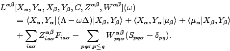
Properties of excited states are defined as derivatives of the excited state energy with respect to an external perturbation. It is advantageous to consider a fully variational Lagrangian of the excited state energy [16],

$$\begin{split}L[X,Y,\Omega,C,Z,W] & = E_{\text{GS}}+ \ensurema... ...} F_{ia} - \sum_{pq} W_{pq} (S_{pq} - \delta_{pq}). \end{split}$$ (7.11)

Here E_GS denotes the ground state energy, F and S are the Fock and overlap matrices, respectively, and indices p, q run over all, occupied and virtual MOs.

First, L is made stationary with respect to all its parameters. The additional Lagrange multipliers Z and W enforce that the MOs satisfy the ground state HF/KS equations and are orthonormal. Z is the so-called Z-vector, while W turns out to be the excited state energy-weighted density matrix. Computation of Z and W requires the solution of a single static TDHF/TDKS response equation (7.4), also called coupled and perturbed HF/KS equation. Once the relaxed densities have been computed, excited state properties are obtained by simple contraction with derivative integrals in the atomic orbital (AO) basis. Thus, computation of excited state gradients is more expensive than that of ground state gradients only by a constant factor which is usually in the range of 1…4.

TDHF/TDDFT expressions for components of the frequency-dependent polarizability α_αβ(ω) can also be reformulated as variational polarizability Lagrangians [81]

$$\begin{split}L^{\alpha\beta} & [X_{\alpha},Y_{\alpha},X_{\bet... ...lpha\beta}_{pq\sigma} (S_{pq\sigma} - \delta_{pq}). \end{split}$$ (7.12)

The stationary point of L^αβ(ω) equals to - α_αβ(ω). The requirement that L^αβ(ω) be stationary with respect to all variational parameters determines the Lagrange multipliers Z^αβ and W^αβ. All polarizability components αβ are processed simultaneously which allows for computation of polarizability derivatives at the computational cost which is only 2-3 higher than for the electronic polarizability itself.